w/ Dalton Craig

For my Rigorous Software Specification and Testing class, Dalton and I decided that we were going to build a quantum simulator and test it using IBMQ's Qiskit library using Python.
The concept was simple enough. We built a two-qubit simulator that used matrix multiplication and kronecker products to make computations on the system. Every statevector would be a one-by-four matrix followed by a toggle state, and each gate would be a four-by-four matrix. For single qubit operations like Hadamard and Pauli-X, the gates would be kroneckered by the identity matrix to create another four-by-four to act on a target qubit.
You can see our presentation slides here:
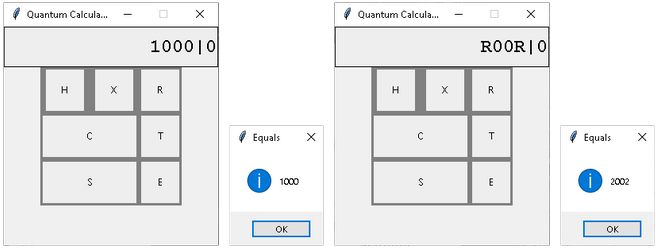
Once we had the gates and the initial statevector with its toggle state established, it was time to develop a mapping system such that we could have symbols to represent the values in the statevector. This was only possible because we limited our operations to Hadamard, Pauli-X, Controlled-Not, and Swap (excluding toggle, reset, and pseudo-measurement).
The mechanics behind single-qubit operations on a multi-qubit register is that the operation is equivalent to the gate tensored with the identity matrix at the same position of the target qubit. For example, if I wanted to apply Hadamard to the first qubit in a two-qubit register \(R\), I would take \(H \otimes I\) and multiply it by the register's statevector.
$$ \left( H \otimes I \right) \left( R \right) = \left(\sqrt{\frac{1}{2}} \begin{pmatrix} 1 & 1 \\ 1 & -1 \end{pmatrix} \otimes \begin{pmatrix} 1 & 0 \\ 0 & 1 \end{pmatrix} \right) \begin{pmatrix} 1 \\ 0 \\ 0 \\ 0 \end{pmatrix} $$
$$ \sqrt{\frac{1}{2}} \begin{pmatrix} 1 & 0 & 1 & 0 \\ 0 & 1 & 0 & 1 \\ 1 & 0 & -1 & 0 \\ 0 & 1 & 0 & -1 \end{pmatrix} \begin{pmatrix} 1 \\ 0 \\ 0 \\ 0 \end{pmatrix} = \sqrt{\frac{1}{2}} \begin{pmatrix} 1 \\ 0 \\ 1 \\ 0 \end{pmatrix} = \begin{pmatrix} \sqrt{\frac{1}{2}} \\ 0 \\ \sqrt{\frac{1}{2}} \\ 0 \end{pmatrix} $$
However, if we wanted to target the second qubit in the register, we would flip the tensor such that the statevector multiplies \(I \otimes H\).
$$ \left( I \otimes H \right) \left( R \right) = \left( \begin{pmatrix} 1 & 0 \\ 0 & 1 \end{pmatrix} \otimes \sqrt{\frac{1}{2}} \begin{pmatrix} 1 & 1 \\ 1 & -1 \end{pmatrix} \right) \begin{pmatrix} 1 \\ 0 \\ 0 \\ 0 \end{pmatrix} $$
$$ \sqrt{\frac{1}{2}} \begin{pmatrix} 1 & 1 & 0 & 0 \\ 1 & -1 & 0 & 0 \\ 0 & 0 & 1 & 1 \\ 0 & 0 & 1 & -1 \end{pmatrix} \begin{pmatrix} 1 \\ 0 \\ 0 \\ 0 \end{pmatrix} = \sqrt{\frac{1}{2}} \begin{pmatrix} 1 \\ 1 \\ 0 \\ 0 \end{pmatrix} = \begin{pmatrix} \sqrt{\frac{1}{2}} \\ \sqrt{\frac{1}{2}} \\ 0 \\ 0 \end{pmatrix} $$
Now that we have shared some about the actual math and concepts driving the program, the needed groundwork is there to discuss how we took these concepts and created a quantum simulator.
What is the first step when creating a program? Some may answer that you must first decide a language to program in, some others may argue that you must first decide the platform to release on, and others may argue that you must prepare the development environment. While those are all valid concerns to have before putting code on your machine, Levi and I subscribe to the school of thought that just knowing what you want to program isn’t enough. While we knew we wanted to create a quantum simulator, simply knowing that doesn’t afford enough understanding of the project to come close to creating good, clean code on a solid structure immediately.
We first needed to carefully define exactly what a quantum simulator is in regards to what we are creating and we needed to explicitly state the expected and required behaviors. For example, we needed to decide if we were going to simulate the actual value of a qubit or the probability of a value for a given qubit. We also had to first decide how many qubits and what operations we wanted our program to use. This provides us with a detailed explanation of the program and some of it’s more major inner-workings; with this we no longer would be programming a black box, something largely unknown to us till we defined it in code.
That’s a great first step, however, we agreed that there is even more that can be done. We wanted to use a linear software model approach to help us better define the structure of the program before we ever wrote a line of code.
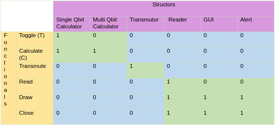
To do this, we needed only one very basic tool, a spreadsheet. You could even use a .csv file. Then we just map all of the major structural components across the horizontal axis and all of the functional components across the vertical axis. Each structural item (a structor) is something roughly akin to a class and a functional object (a functional) is akin to a method or function within a class. This creates a grid where each intersection can represent the relationship between a functional and a structor. For each intersection, you place a \(1\) if the structor has that functional and a \(0\) or nothing if it does not.
The goal with this exercise is to rearrange and consolidate elements in the set of structors and functionals such that you can gain a good understanding of the natural grouping of the major elements in the program. The commonly accepted most efficient form you want your model to finish in is called block diagonal. In a block diagonal model, your model is perfectly square (same number of structors and functionals) and every \(1\) in the table runs diagonally through the table from top left to bottom right. This shows a low level of unnecessary coupling between elements which makes your program more modular and easier to maintain or edit later. This model is called a modularity matrix.
Our first iteration of the modularity matrix was a mess. It contained too much information, including some stuff that was entirely irrelevant to a modularity matrix (some data structors which would never have any functionals). By removing overly redundant elements, elements that aren’t actually useful in a modularity matrix, and by abstracting several elements into single more encompassing elements we were able to create a perfectly block diagonal modularity matrix that made creating the program and its respective elements much easier. You can see it below.
While the modularity matrix is a useful tool, it should be noted that it is only good for exposing flaws in your structure of a program and for giving you a recommended roadmap. Your modularity matrix may not always be the best approach as you may learn something you thought would be complex and need to be broken into separate structurs/classes is actually much easier. We have a good example: our matrix has multi-qubit calculator and single-qubit calculator structors when our code ended up being simpler than expected for this and we only implemented a single calculator class. Breaking it into two classes here would have added undue complication and repetition.